from classy import Class
# create instance of the class "Class"
LambdaCDM = Class()
# pass input parameters
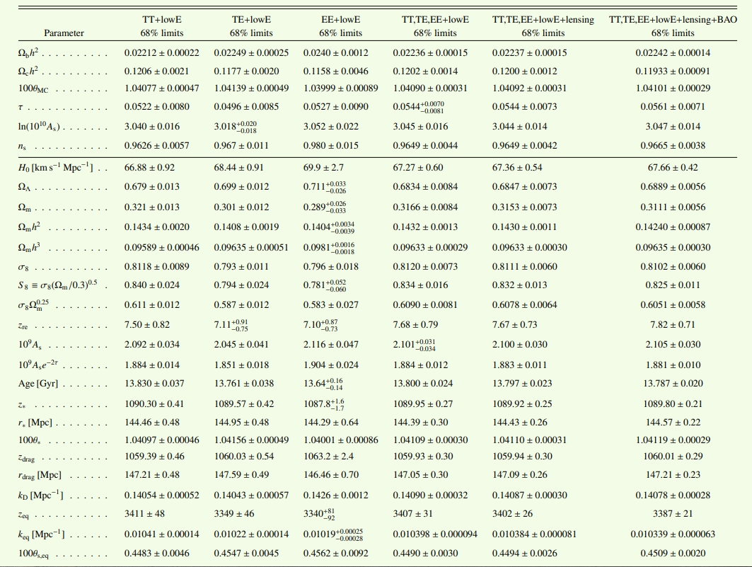
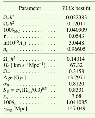
LambdaCDM.set({'omega_b':0.02242,'omega_cdm':0.11933,'h':0.6766,'A_s':2.105e-09,'n_s':0.9665,'tau_reio':0.0561})
LambdaCDM.set({'output':'mPk','P_k_max_h/Mpc':4.0})
# run class
LambdaCDM.compute()
import numpy as np
kk = np.logspace(-4,np.log10(4),600) # k in h/Mpc
Pk = [] # P(k) in (Mpc/h)**3
h = LambdaCDM.h() # get reduced Hubble for conversions to 1/Mpc
for k in kk:
Pk.append(LambdaCDM.pk(k*h,0.)*h**3) # function .pk(k,z)
# uncomment to get plots displayed in notebook
%matplotlib inline
import matplotlib.pyplot as plt
# plot P(k)
plt.figure(2)
plt.xscale('log');plt.yscale('log');plt.xlim(kk[0],kk[-1])
plt.xlabel(r'$k \,\,\,\, [h/\mathrm{Mpc}]$')
plt.ylabel(r'$P(k) \,\,\,\, [\mathrm{Mpc}/h]^3$')
plt.plot(kk,Pk,'b-')
import numpy as np
parameters = '_'.join([f"{key}_{value:.3f}" for key, value in list(LambdaCDM.pars.items())[:3]])
filename = f"data_Omega0_m_{LambdaCDM.Omega0_m():.3f}_h_{LambdaCDM.h():.3f}.txt"
with open(filename, 'w') as file:
for a, b in zip(kk, Pk):
file.write(f"{a} {b}\n")
Smilie Vote is loading.
%config InlineBackend.figure_format = ‘retina’
import matplotlib.pyplot as plt
import numpy as np
from scipy.interpolate import interp1d
import matplotlib
font = {‘size’ : 13, ‘family’:’STIXGeneral’}
axislabelfontsize=’large’
matplotlib.rc(‘font’, **font)
fig = plt.figure(figsize = (4,4))
left, bottom, width, height = 0.0,-0.4,1.4,0.6
ax0 = fig.add_axes([left,bottom,width,height])
plt.xticks([])
plt.yticks([])
################################
left, bottom, width, height = 0.,0.0,1.4,0.6
ax2 = fig.add_axes([left,bottom,width,height])
ax2.plot(kk,Pk_lcdm,’g-‘,label=r’$\Lambda$CDM’)
ax2.plot(kk,Pk,’r–‘,label=’PUDF’)
ax2.set_yscale(‘log’)
ax2.set_xscale(‘log’)
ax2.set_xlim(kk[0],kk[-1])
ax2.set_xticks([])
plt.legend()
plt.ylabel(r’$P(k) \,\,\,\, [\mathrm{Mpc}/h]^3$’)
################################
left, bottom, width, height = 0.0,-0.4,1.4,0.4
ax11 = fig.add_axes([left,bottom,width,height])
ax11.plot(kk,(np.array(Pk)-np.array(Pk_lcdm))/np.array(Pk_lcdm))
ax11.set_xscale(‘log’)
ax11.set_xlim(kk[0],kk[-1])
ax11.set_xlabel(r’$k \,\,\,\, [h/\mathrm{Mpc}]$’)
plt.ylabel(r’$P(k)_\mathrm{PUDF}/P(k)_\mathrm{\Lambda CDM} – 1$’,fontsize=10)
#############################
plt.savefig(‘Pk.pdf’,bbox_inches = ‘tight’)
plt.show()